Illustration of Jacobi Fields

This tutorial illustrates the usage of Jacobi Fields within Manopt.jl. For this tutorial you should be familiar with the basic terminology on a manifold like the exponential and logarithmic map as well as shortest geodesics.

We first initialize the manifold

using Manopt, Manifolds

and we define some colors from Paul Tol

using Colors
black = RGBA{Float64}(colorant"#000000")
TolVibrantOrange = RGBA{Float64}(colorant"#EE7733")
TolVibrantCyan = RGBA{Float64}(colorant"#33BBEE")
TolVibrantTeal = RGBA{Float64}(colorant"#009988")

Assume we have two points on the equator of the Sphere $\mathcal M = \mathbb S^2$

M = Sphere(2)
p, q = [[1.0, 0.0, 0.0], [0.0, 1.0, 0.0]]

2-element Array{Array{Float64,1},1}:
 [1.0, 0.0, 0.0]
 [0.0, 1.0, 0.0]

their connecting shortest geodesic (sampled at 100 points)

geodesicCurve = shortest_geodesic(M, p, q, [0:0.1:1.0...]);

looks as follows using the asymptote_export_S2_signals export

asymptote_export_S2_signals("jacobiGeodesic.asy";
    render = asyResolution,
    curves=[geodesicCurve], points = [ [x,y] ],
    colors=Dict(:curves => [black], :points => [TolVibrantOrange]),
    dot_size = 3.5, line_width = 0.75, camera_position = (1.,1.,.5)
)
render_asymptote("jacobiGeodesic.asy"; render = 2)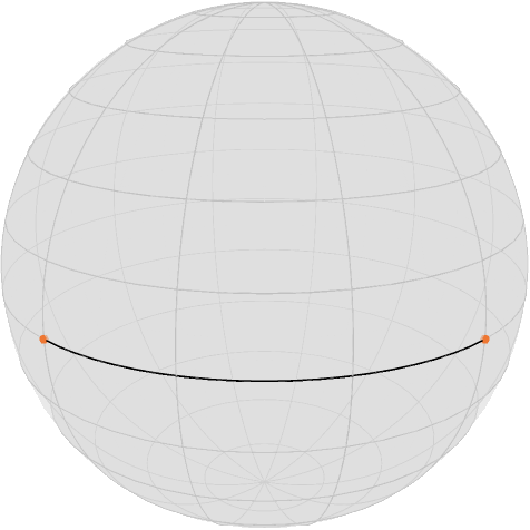

A geodesic connecting two points on the equator

where $x$ is on the left. Then this tutorial solves the following task:

Given a direction $X_p∈ T_x\mathcal M$, for example

X = [0.0, 0.4, 0.5]

3-element Array{Float64,1}:
 0.0
 0.4
 0.5

we move the start point $x$ into, how does any point on the geodesic move?

Or mathematically: Compute $D_p g(t; p,q)$ for some fixed $t∈[0,1]$ and a given direction $X_p$. Of course two cases are quite easy: For $t=0$ we are in $x$ and how $x$ “moves” is already known, so $D_x g(0;p,q) = X$. On the other side, for $t=1$, $g(1; p,q) = q$ which is fixed, so $D_p g(1; p,q)$ is the zero tangent vector (in $T_q\mathcal M$).

For all other cases we employ a jacobi_field, which is a (tangent) vector field along the shortest geodesic given as follows: The geodesic variation $\Gamma_{g,X}(s,t)$ is defined for some $\varepsilon > 0$ as

\[\Gamma_{g,X}(s,t):=\exp{\gamma_{p,X}(s)}[t\log_{g(s;p,X)}p],\qquad s∈(-\varepsilon,\varepsilon),\ t∈[0,1].\]

Intuitively we make a small step $s$ into direction $\xi$ using the geodesic $g(\cdot; p,X)$ and from $r=g(s; p,X)$ we follow (in $t$) the geodesic $g(\cdot; r,q)$. The corresponding Jacobi field $J_{g,X}$ along $g(\cdot; p,q)$ is given by

\[J_{g,X}(t):=\frac{D}{\partial s}\Gamma_{g,X}(s,t)\Bigl\rvert_{s=0}\]

which is an ODE and we know the boundary conditions $J_{g,X}(0)=X$ and $J_{g,X}(t) = 0$. In symmetric spaces we can compute the solution, since the system of ODEs decouples, see for example do Carmo, Chapter 4.2. Within Manopt.jl this is implemented as jacobi_field(M,p,q,t,X[,β]), where the optional parameter (function) β specifies, which Jacobi field we want to evaluate and the one used here is the default.

We can hence evaluate that on the points on the geodesic at

T = [0:0.1:1.0...]

namely

r = shortest_geodesic(M, p, q, T)

the geodesic moves as

W = jacobi_field.(Ref(M), Ref(p), Ref(q), T, Ref(X))

11-element Array{Array{Float64,1},1}:
 [0.0, 0.4, 0.5]
 [-0.05631640741448312, 0.35556780261424964, 0.4938441702975689]
 [-0.09888543819998319, 0.3043380852144492, 0.47552825814757677]
 [-0.12711733992707308, 0.249481826772743, 0.4455032620941839]
 [-0.14106846055019354, 0.1941640786499874, 0.4045084971874737]
 [-0.1414213562373095, 0.14142135623730953, 0.35355339059327373]
 [-0.1294427190999916, 0.09404564036679572, 0.29389262614623657]
 [-0.10692078290260418, 0.05447885996874562, 0.2269952498697734]
 [-0.07608452130361228, 0.024721359549995783, 0.15450849718747367]
 [-0.039507533623805505, 0.006257378601609233, 0.07821723252011542]
 [0.0, 0.0, 0.0]

which can also be called using differential_geodesic_startpoint. We can add to the image above by creating extended tangent vectors the include their base points

V = [Tuple([a, b]) for (a, b) in zip(r, W)]

11-element Array{Tuple{Array{Float64,1},Array{Float64,1}},1}:
 ([1.0, 0.0, 0.0], [0.0, 0.4, 0.5])
 ([0.9876883405951378, 0.15643446504023087, 0.0], [-0.05631640741448312, 0.35556780261424964, 0.4938441702975689])
 ([0.9510565162951535, 0.3090169943749474, 0.0], [-0.09888543819998319, 0.3043380852144492, 0.47552825814757677])
 ([0.8910065241883679, 0.45399049973954675, 0.0], [-0.12711733992707308, 0.249481826772743, 0.4455032620941839])
 ([0.8090169943749475, 0.5877852522924731, 0.0], [-0.14106846055019354, 0.1941640786499874, 0.4045084971874737])
 ([0.7071067811865476, 0.7071067811865475, 0.0], [-0.1414213562373095, 0.14142135623730953, 0.35355339059327373])
 ([0.5877852522924731, 0.8090169943749475, 0.0], [-0.1294427190999916, 0.09404564036679572, 0.29389262614623657])
 ([0.45399049973954686, 0.8910065241883678, 0.0], [-0.10692078290260418, 0.05447885996874562, 0.2269952498697734])
 ([0.30901699437494745, 0.9510565162951536, 0.0], [-0.07608452130361228, 0.024721359549995783, 0.15450849718747367])
 ([0.15643446504023092, 0.9876883405951378, 0.0], [-0.039507533623805505, 0.006257378601609233, 0.07821723252011542])
 ([6.123233995736766e-17, 1.0, 0.0], [0.0, 0.0, 0.0])

and add that as one further set to the Asymptote export.

asymptote_export_S2_signals("jacobiGeodesicdifferential_geodesic_startpoint.asy";
    render = asyResolution,
    curves=[geodesicCurve], points = [ [x,y], Z], tangent_vectors = [Vx],
    colors=Dict(
        :curves => [black],
        :points => [TolVibrantOrange,TolVibrantCyan],
        :tvectors => [TolVibrantCyan]
    ),
    dot_sizes = [3.5,2.], line_width = 0.75, camera_position = (1.,1.,.5)
)
render_asymptote("jacobiGeodesicdifferential_geodesic_startpoint.asy"; render = 2)

$A Jacobi field for \$D_xg(t,x,y)[\\eta]\$$

If we further move the end point, too, we can derive that Differential in direction

Xq = [0.2, 0.0, -0.5]
W2 = differential_geodesic_endpoint.(Ref(M), Ref(p), Ref(q), T, Ref(Xq))
V2 = [Tuple([a, b]) for (a, b) in zip(r, W2)]

11-element Array{Tuple{Array{Float64,1},Array{Float64,1}},1}:
 ([1.0, 0.0, 0.0], [0.0, -0.0, 0.0])
 ([0.9876883405951378, 0.15643446504023087, 0.0], [0.0031286893008046165, -0.019753766811902752, -0.07821723252011542])
 ([0.9510565162951535, 0.3090169943749474, 0.0], [0.012360679774997892, -0.03804226065180614, -0.15450849718747367])
 ([0.8910065241883679, 0.45399049973954675, 0.0], [0.02723942998437282, -0.053460391451302075, -0.2269952498697734])
 ([0.8090169943749475, 0.5877852522924731, 0.0], [0.04702282018339786, -0.0647213595499958, -0.29389262614623657])
 ([0.7071067811865476, 0.7071067811865475, 0.0], [0.07071067811865477, -0.07071067811865475, -0.35355339059327373])
 ([0.5877852522924731, 0.8090169943749475, 0.0], [0.0970820393249937, -0.07053423027509677, -0.4045084971874737])
 ([0.45399049973954686, 0.8910065241883678, 0.0], [0.1247409133863715, -0.06355866996353654, -0.4455032620941839])
 ([0.30901699437494745, 0.9510565162951536, 0.0], [0.1521690426072246, -0.04944271909999159, -0.47552825814757677])
 ([0.15643446504023092, 0.9876883405951378, 0.0], [0.17778390130712482, -0.028158203707241553, -0.4938441702975689])
 ([6.123233995736766e-17, 1.0, 0.0], [0.2, 0.0, -0.5])

and we can combine both keeping the base point

V3 = [Tuple([a, b]) for (a, b) in zip(r, W2 + W)]

11-element Array{Tuple{Array{Float64,1},Array{Float64,1}},1}:
 ([1.0, 0.0, 0.0], [0.0, 0.4, 0.5])
 ([0.9876883405951378, 0.15643446504023087, 0.0], [-0.053187718113678506, 0.33581403580234687, 0.41562693777745346])
 ([0.9510565162951535, 0.3090169943749474, 0.0], [-0.0865247584249853, 0.26629582456264306, 0.3210197609601031])
 ([0.8910065241883679, 0.45399049973954675, 0.0], [-0.09987790994270027, 0.19602143532144092, 0.2185080122244105])
 ([0.8090169943749475, 0.5877852522924731, 0.0], [-0.09404564036679568, 0.12944271909999158, 0.11061587104123716])
 ([0.7071067811865476, 0.7071067811865475, 0.0], [-0.07071067811865474, 0.07071067811865478, 0.0])
 ([0.5877852522924731, 0.8090169943749475, 0.0], [-0.032360679774997916, 0.02351141009169895, -0.11061587104123716])
 ([0.45399049973954686, 0.8910065241883678, 0.0], [0.01782013048376732, -0.009079809994790917, -0.2185080122244105])
 ([0.30901699437494745, 0.9510565162951536, 0.0], [0.07608452130361233, -0.024721359549995804, -0.3210197609601031])
 ([0.15643446504023092, 0.9876883405951378, 0.0], [0.1382763676833193, -0.02190082510563232, -0.41562693777745346])
 ([6.123233995736766e-17, 1.0, 0.0], [0.2, 0.0, -0.5])

asymptote_export_S2_signals("jacobiGeodesicResult.asy";
   render = asyResolution,
   curves=[geodesicCurve], points = [ [x,y], Z], tangent_vectors = [Vx,Vy,Vb],
   colors=Dict(
       :curves => [black],
       :points => [TolVibrantOrange,TolVibrantCyan],
       :tvectors => [TolVibrantCyan,TolVibrantCyan,TolVibrantTeal]
  ),
  dot_sizes = [3.5,2.], line_width = 0.75, camera_position = (1.,1.,0.)
)
render_asymptote("jacobiGeodesicResult.asy"; render = 2)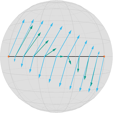

A Jacobi field for the effect of two differentials (blue) in sum (teal)

Literature

[doCarmo1992] do Carmo, M. P.: Riemannian Geometry, Mathematics: Theory & Applications, Birkhäuser Basel, 1992, ISBN: 0-8176-3490-8
[BergmannGousenbourger2018] Bergmann, R.; Gousenbourger, P.-Y.: A variational model for data fitting on manifolds by minimizing the acceleration of a Bézier curve, Frontiers in Applied Mathematics and Statistics, 2018. doi: 10.3389/fams.2018.00059