Get started: Optimize!

This example illustrates how to set up and solve optimization problems and how to further get data from the algorithm using DebugOptions and RecordOptions

To start from the quite general case: A Solver is an algorithm that aims to solve

\[\operatorname*{argmin}_{x∈\mathcal M} f(x)\]

where $\mathcal M$ is a Manifold and $f\colon\mathcal M \to \mathbb R$ is the cost function.

In Manopt.jl a Solver is an algorithm that requires a Problem p and Options o. While former contains static data, most prominently the manifold $\mathcal M$ (usually as p.M) and the cost function $f$ (usually as p.cost), the latter contains dynamic data, i.e. things that usually change during the algorithm, are allowed to change, or specify the details of the algorithm to use. Together they form a plan. A plan uniquely determines the algorithm to use and provide all necessary information to run the algorithm.

Example

A gradient plan consists of a GradientProblem with the fields M, cost function $f$ as well as gradient storing the gradient function corresponding to $f$. Accessing both functions can be done directly but should be encapsulated using get_cost(p,x) and get_gradient(p,x), where in both cases x is a point on the Manifold M. Second, the GradientDescentOptions specify that the algorithm to solve the GradientProblem will be the gradient descent algorithm. It requires an initial value o.x0, a StoppingCriterion o.stop, a Stepsize o.stepsize and a retraction o.retraction and it internally stores the last evaluation of the gradient at o.∇ for convenience. The only mandatory parameter is the initial value x0, though the defaults for both the stopping criterion (StopAfterIteration(100)) as well as the stepsize (ConstantStepsize(1.) are quite conservative, but are chosen to be as simple as possible.

With these two at hand, running the algorithm just requires to call x_opt = solve(p,o).

In the following two examples we will see, how to use a higher level interface that allows to more easily activate for example a debug output or record values during the iterations

The given Dataset

using Manopt, Manifolds
using Random, Colors

For a persistent random set we use

n = 100
σ = π / 8
M = Sphere(2)
x = 1 / sqrt(2) * [1.0, 0.0, 1.0]
Random.seed!(42)
data = [exp(M, x, random_tangent(M, x, Val(:Gaussian), σ)) for i in 1:n]

and we define some colors from Paul Tol

black = RGBA{Float64}(colorant"#000000")
TolVibrantOrange = RGBA{Float64}(colorant"#EE7733")
TolVibrantBlue = RGBA{Float64}(colorant"#0077BB")
TolVibrantTeal = RGBA{Float64}(colorant"#009988")
TolVibrantMagenta = RGBA{Float64}(colorant"#EE3377")

Then our data rendered using asymptote_export_S2_signals looks like

asymptote_export_S2_signals("startDataAndCenter.asy";
    points = [ [x], data],
    colors=Dict(:points => [TolVibrantBlue, TolVibrantTeal]),
    dot_size = 3.5, camera_position = (1.,.5,.5)
)
render_asymptote("startDataAndCenter.asy"; render = 2)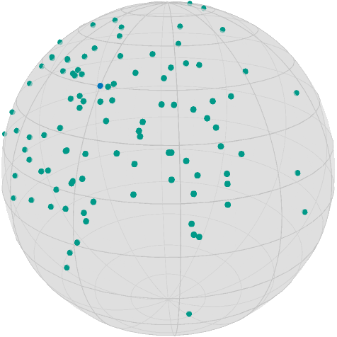

$The data of noisy versions of \$x\$$

Computing the Mean

To compute the mean on the manifold we use the characterization, that the Euclidean mean minimizes the sum of squared distances, and end up with the following cost function. Its minimizer is called Riemannian Center of Mass.

F = y -> sum(1 / (2 * n) * distance.(Ref(M), Ref(y), data) .^ 2)
∇F = y -> sum(1 / n * ∇distance.(Ref(M), data, Ref(y)))

note that the ∇distance defaults to the case p=2, i.e. the gradient of the squared distance. For details on convergence of the gradient descent for this problem, see [Afsari, Tron, Vidal, 2013]

The easiest way to call the gradient descent is now to call gradient_descent

xMean = gradient_descent(M, F, ∇F, data[1])

but in order to get more details, we further add the debug= options, which act as a decorator pattern using the DebugOptions and DebugActions. The latter store values if that's necessary, for example for the DebugChange that prints the change during the last iteration. The following debug prints

# i | x: | Last Change: | F(x):`

as well as the reason why the algorithm stopped at the end. Here, the format shorthand and the [DebugFactory] are used, which returns a DebugGroup of DebugAction performed each iteration and the stop, respectively.

xMean = gradient_descent(
    M,
    F,
    ∇F,
    data[1];
    debug=[:Iteration, " | ", :x, " | ", :Change, " | ", :Cost, "\n", :Stop],
)

Initial | x: [0.5737338264338113, -0.1728651513118652, 0.8005917410687816] |  | F(x): 0.22606088442202987
# 1 | x: [0.7823885991620455, 0.08556904440746377, 0.6168841208366815] | Last Change: 0.38188652881305873 | F(x): 0.14924728281088784
# 2 | x: [0.7917377109136624, 0.09720922045898238, 0.603076914311061] | Last Change: 0.020335997468986768 | F(x): 0.14902948995714224
# 3 | x: [0.792283271084327, 0.0977159913287459, 0.6022780117176446] | Last Change: 0.001092107177300155 | F(x): 0.14902886086292993
# 4 | x: [0.7923155575566623, 0.0977379000751398, 0.6022319819991105] | Last Change: 6.034190038620069e-5 | F(x): 0.14902885894006118
# 5 | x: [0.7923174650259398, 0.09773883592992508, 0.6022293205797368] | Last Change: 3.4056244498865836e-6 | F(x): 0.14902885893393145
# 6 | x: [0.7923175775065069, 0.09773887521445883, 0.6022291662199968] | Last Change: 1.971238338250365e-7 | F(x): 0.14902885893391132
# 7 | x: [0.7923175841297168, 0.09773887682107817, 0.6022291572454814] | Last Change: 3.332000937312528e-8 | F(x): 0.1490288589339113
The algorithm reached approximately critical point; the gradient norm (6.549992173466581e-10) is less than 1.0e-8.

asymptote_export_S2_signals("startDataCenterMean.asy";
    points = [ [x], data, [xMean] ],
    colors=Dict(:points => [TolVibrantBlue, TolVibrantTeal, TolVibrantOrange]),
    dot_size = 3.5, camera_position = (1.,.5,.5)
)
render_asymptote("startDataCenterMean.asy"; render = 2)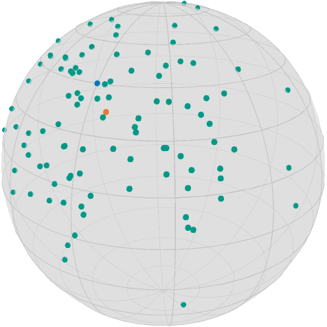

The resulting mean (orange)

Computing the Median

Similar to the mean you can also define the median as the minimizer of the distances, see for example [Bačák, 2014], but since this problem is not differentiable, we employ the Cyclic Proximal Point (CPP) algorithm, described in the same reference. We define

F2 = y -> sum(1 / (2 * n) * distance.(Ref(M), Ref(y), data))
proxes = Function[(λ, y) -> prox_distance(M, λ / n, di, y, 1) for di in data]

where the Function is a helper for global scope to infer the correct type.

We then call the cyclic_proximal_point as

o = cyclic_proximal_point(
    M,
    F2,
    proxes,
    data[1];
    debug=[:Iteration, " | ", :x, " | ", :Change, " | ", :Cost, "\n", 50, :Stop],
    record=[:Iteration, :Change, :Cost],
    return_options=true,
)
xMedian = get_solver_result(o)
values = get_record(o)

Initial | x: [0.5737338264338113, -0.1728651513118652, 0.8005917410687816] |  | F(x): 0.2986800793934701
# 50 | x: [0.7897340334179458, 0.07829927185150312, 0.608431902918448] | Last Change: 0.08025247706840972 | F(x): 0.2454542345696772
# 100 | x: [0.7899680461384707, 0.0786029490954357, 0.6080888606722517] | Last Change: 0.0004925110930805728 | F(x): 0.24545405097297035
# 150 | x: [0.790036413163267, 0.07868191382352602, 0.6079898208960562] | Last Change: 0.00013941286404552968 | F(x): 0.2454540279144726
# 200 | x: [0.7900676764403393, 0.0787154178585569, 0.6079448573970901] | Last Change: 6.242300783602185e-5 | F(x): 0.24545402161497565
# 250 | x: [0.7900851818616217, 0.07873311977053307, 0.6079198148226581] | Last Change: 3.43990845233452e-5 | F(x): 0.2454540191973801
The algorithm performed a step with a change (0.0) less than 1.0e-12.

where the differences to gradient_descent are as follows

the third parameter is now an Array of proximal maps
debug is reduces to only every 50th iteration
we further activated a RecordAction using the record= optional parameter. These work very similar to those in debug, but they collect their data in an array. The high level interface then returns two variables; the values do contain an array of recorded datum per iteration. Here a Tuple containing the iteration, last change and cost respectively; see RecordGroup, RecordIteration, RecordChange, RecordCost as well as the RecordFactory for details. The values contains hence a tuple per iteration, that itself consists of (by order of specification) the iteration number, the last change and the cost function value.

These recorded entries read

values

254-element Array{Tuple{Int64,Float64,Float64},1}:
 (1, 0.30579511191461684, 0.24765709821769438)
 (2, 0.03915137245269646, 0.24599998171726192)
 (3, 0.014699094618098311, 0.24568197834842026)
 (4, 0.0075130396403671924, 0.24557305929190362)
 (5, 0.0044893480449786525, 0.2455249161082335)
 (6, 0.002953601317596155, 0.24550007064482607)
 (7, 0.0020748587403644106, 0.2454858341409571)
 (8, 0.0015286431209686094, 0.2454770356861027)
 (9, 0.001167743288968188, 0.24547127727824164)
 (10, 0.0009178169876077584, 0.24546733510439248)
 ⋮
 (246, 3.175031505921871e-7, 0.24545401932704825)
 (247, 2.976504617249705e-7, 0.24545401929389432)
 (248, 2.846862848779986e-7, 0.24545401926124036)
 (249, 2.669762502188827e-7, 0.24545401922907212)
 (250, 2.269677253324963e-7, 0.2454540191973801)
 (251, 1.659323085197815e-7, 0.24545401916615991)
 (252, 1.0745380149674388e-7, 0.24545401913540657)
 (253, 7.300048299977716e-8, 0.24545401910510922)
 (254, 0.0, 0.24545401907525016)

The resulting median and mean for the data hence are

asymptote_export_S2_signals("startDataCenterMean.asy";
    points = [ [x], data, [xMean], [xMedian] ],
    colors=Dict(:points => [TolVibrantBlue, TolVibrantTeal, TolVibrantOrange, TolVibrantMagenta]),
    dot_size = 3.5, camera_position = (1.,.5,.5)
)
render_asymptote("startDataCenterMedianAndMean.asy"; render = 2)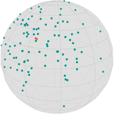

The resulting mean (orange) and median (magenta)

Literature

[Bačák, 2014] Bačák, M: Computing Medians and Means in Hadamard Spaces., SIAM Journal on Optimization, Volume 24, Number 3, pp. 1542–1566, doi: 10.1137/140953393, arxiv: 1210.2145.
[Afsari, Tron, Vidal, 2013] Afsari, B; Tron, R.; Vidal, R.: On the Convergence of Gradient Descent for Finding the Riemannian Center of Mass, SIAM Journal on Control and Optimization, Volume 51, Issue 3, pp. 2230–2260. doi: 10.1137/12086282X, arxiv: 1201.0925